install.packages(c("tidyverse", "nycflights13"))Data Merging
Set up
To complete this session, you need to load in the following R packages:
Install packages
To install new R packages, run the following (excluding the packages you have already installed):
Introduction
We often need to append or join multiple data sets to one another. Perhaps you got data from multiple different sources and you want to run analyses across them. Or you collected your data across different time periods and want to join them all together for your research. In this session, we will learn some helpful tools for doing this common task.
Let’s get started!
Keys
To join multiple tables together, you need a key. These are common values across the two data sets that allow them to be connected.
A primary key uniquely identifies each observation within your data set. For example, each airline in the airlines data set in the nycflights13 R package can be identified by its two letter carrier code, which is stored in the carrier variable:
airlines# A tibble: 16 × 2
carrier name
<chr> <chr>
1 9E Endeavor Air Inc.
2 AA American Airlines Inc.
3 AS Alaska Airlines Inc.
4 B6 JetBlue Airways
5 DL Delta Air Lines Inc.
6 EV ExpressJet Airlines Inc.
7 F9 Frontier Airlines Inc.
8 FL AirTran Airways Corporation
9 HA Hawaiian Airlines Inc.
10 MQ Envoy Air
11 OO SkyWest Airlines Inc.
12 UA United Air Lines Inc.
13 US US Airways Inc.
14 VX Virgin America
15 WN Southwest Airlines Co.
16 YV Mesa Airlines Inc. Sometimes you need to use multiple variables to uniquely identify your observations. This is particularly common when using time-series data (for example, country-year, or leader-year). For example, observations in the weather data set, which provides information about the hourly weather across New York City’s airports, are uniquely identified by the airport (origin) and time the weather was recorded (time_hour):
weather# A tibble: 26,115 × 15
origin year month day hour temp dewp humid wind_dir wind_speed
<chr> <int> <int> <int> <int> <dbl> <dbl> <dbl> <dbl> <dbl>
1 EWR 2013 1 1 1 39.0 26.1 59.4 270 10.4
2 EWR 2013 1 1 2 39.0 27.0 61.6 250 8.06
3 EWR 2013 1 1 3 39.0 28.0 64.4 240 11.5
4 EWR 2013 1 1 4 39.9 28.0 62.2 250 12.7
5 EWR 2013 1 1 5 39.0 28.0 64.4 260 12.7
6 EWR 2013 1 1 6 37.9 28.0 67.2 240 11.5
7 EWR 2013 1 1 7 39.0 28.0 64.4 240 15.0
8 EWR 2013 1 1 8 39.9 28.0 62.2 250 10.4
9 EWR 2013 1 1 9 39.9 28.0 62.2 260 15.0
10 EWR 2013 1 1 10 41 28.0 59.6 260 13.8
# ℹ 26,105 more rows
# ℹ 5 more variables: wind_gust <dbl>, precip <dbl>, pressure <dbl>,
# visib <dbl>, time_hour <dttm>We can verify that each observation has a unique value as its primary key using count() and filter():
# A tibble: 0 × 2
# ℹ 2 variables: carrier <chr>, n <int># A tibble: 0 × 3
# ℹ 3 variables: time_hour <dttm>, origin <chr>, n <int>If you know that each row of your data set is a unique observation, you can create your own primary key using its row number:
airlines |>
  mutate(id = row_number(), .before = 1)
# A tibble: 16 × 3
id carrier name
<int> <chr> <chr>
1 1 9E Endeavor Air Inc.
2 2 AA American Airlines Inc.
3 3 AS Alaska Airlines Inc.
4 4 B6 JetBlue Airways
5 5 DL Delta Air Lines Inc.
6 6 EV ExpressJet Airlines Inc.
7 7 F9 Frontier Airlines Inc.
8 8 FL AirTran Airways Corporation
9 9 HA Hawaiian Airlines Inc.
10 10 MQ Envoy Air
11 11 OO SkyWest Airlines Inc.
12 12 UA United Air Lines Inc.
13 13 US US Airways Inc.
14 14 VX Virgin America
15 15 WN Southwest Airlines Co.
16 16 YV Mesa Airlines Inc. Basic joins
Primary keys serve as your connection to foreign keys, which are the variables that allow you to uniquely identify observations within the data set you want to join to your original data set. For example, flights$carrier is a foreign key that connects to the primary key airlines$carrier.
You can join data sets using their primary and foreign keys using one of six join functions provided in the dplyr R package (which is loaded in with tidyverse). These are: left_join(), inner_join(), right_join(), full_join(), semi_join(), and anti_join(). All of these functions take two data frames (which I will refer to as primary and foreign) and return a data frame.
Mutating joins
Mutating joins create new columns by appending information in foreign to primary according to the key and join function you use. There are four mutating join functions: left_join(), right_join(), inner_join(), and full_join().
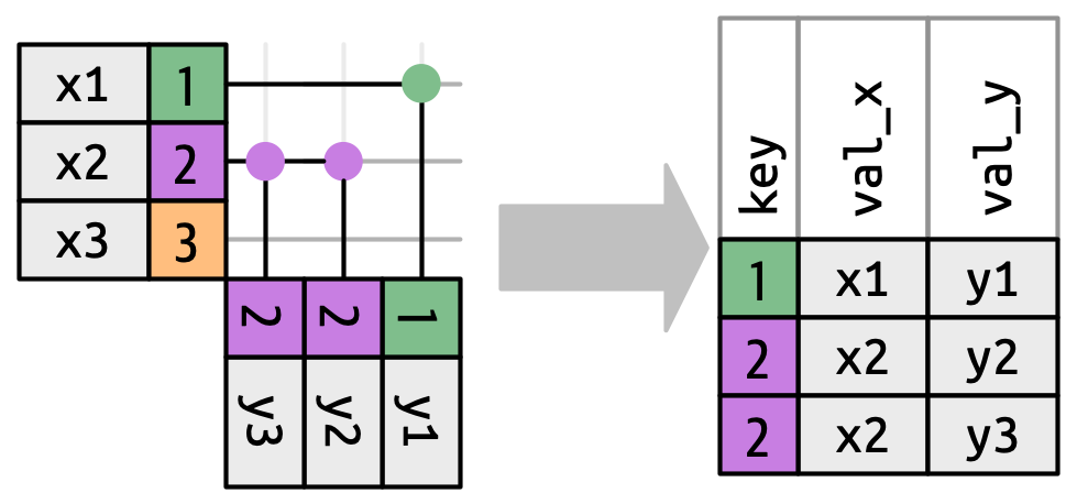
left_join() matches observations in primary and foreign by their keys, then copies all other variables in foreign to primary. The resulting data frame will always have the same number of rows as primary. For example, let’s join flights (which provides information on all flights that departed NYC airports in 2013) with airlines:
flights |>
  left_join(airlines)
# A tibble: 336,776 × 20
year month day dep_time sched_dep_time dep_delay arr_time sched_arr_time
<int> <int> <int> <int> <int> <dbl> <int> <int>
1 2013 1 1 517 515 2 830 819
2 2013 1 1 533 529 4 850 830
3 2013 1 1 542 540 2 923 850
4 2013 1 1 544 545 -1 1004 1022
5 2013 1 1 554 600 -6 812 837
6 2013 1 1 554 558 -4 740 728
7 2013 1 1 555 600 -5 913 854
8 2013 1 1 557 600 -3 709 723
9 2013 1 1 557 600 -3 838 846
10 2013 1 1 558 600 -2 753 745
# ℹ 336,766 more rows
# ℹ 12 more variables: arr_delay <dbl>, carrier <chr>, flight <int>,
# tailnum <chr>, origin <chr>, dest <chr>, air_time <dbl>, distance <dbl>,
# hour <dbl>, minute <dbl>, time_hour <dttm>, name <chr>When you run this in RStudio you will see the following message printed in your console:
Joining with `by = join_by(carrier)`This is letting you know the key left_join() used to match observations in flights with those in airlines. It guessed correctly: we wanted to match these data sets by airline. However, we should not rely on R to guess correctly every time. This can lead to incorrect matches, which can mess up your analysis down the line. Instead, you should always specify the key yourself using the by argument.
# A tibble: 336,776 × 20
    year month   day dep_time sched_dep_time dep_delay arr_time sched_arr_time
   <int> <int> <int>    <int>          <int>     <dbl>    <int>          <int>
 1  2013     1     1      517            515         2      830            819
 2  2013     1     1      533            529         4      850            830
 3  2013     1     1      542            540         2      923            850
 4  2013     1     1      544            545        -1     1004           1022
 5  2013     1     1      554            600        -6      812            837
 6  2013     1     1      554            558        -4      740            728
 7  2013     1     1      555            600        -5      913            854
 8  2013     1     1      557            600        -3      709            723
 9  2013     1     1      557            600        -3      838            846
10  2013     1     1      558            600        -2      753            745
# ℹ 336,766 more rows
# ℹ 12 more variables: arr_delay <dbl>, carrier <chr>, flight <int>,
#   tailnum <chr>, origin <chr>, dest <chr>, air_time <dbl>, distance <dbl>,
# hour <dbl>, minute <dbl>, time_hour <dttm>, name <chr>Here is a visualization of these joins:
If left_join() cannot find a match for a primary key it will fill the values in the new columns created by copying foreign over with NA. For example,
flights |>
  left_join(planes, by = join_by(tailnum, year)) |>
  filter(tailnum == "N3ALAA") |>
  select(tailnum, year, flight, origin, type:engine)
# A tibble: 63 × 11
tailnum year flight origin type manufacturer model engines seats speed
<chr> <int> <int> <chr> <chr> <chr> <chr> <int> <int> <int>
1 N3ALAA 2013 301 LGA <NA> <NA> <NA> NA NA NA
2 N3ALAA 2013 353 LGA <NA> <NA> <NA> NA NA NA
3 N3ALAA 2013 301 LGA <NA> <NA> <NA> NA NA NA
4 N3ALAA 2013 359 LGA <NA> <NA> <NA> NA NA NA
5 N3ALAA 2013 1351 JFK <NA> <NA> <NA> NA NA NA
6 N3ALAA 2013 301 LGA <NA> <NA> <NA> NA NA NA
7 N3ALAA 2013 353 LGA <NA> <NA> <NA> NA NA NA
8 N3ALAA 2013 1351 JFK <NA> <NA> <NA> NA NA NA
9 N3ALAA 2013 1205 EWR <NA> <NA> <NA> NA NA NA
10 N3ALAA 2013 84 JFK <NA> <NA> <NA> NA NA NA
# ℹ 53 more rows
# ℹ 1 more variable: engine <chr>inner_join(), right_join(), and full_join() all work similarly to left_join(). They differ on which rows they keep. left_join() kept the rows in primary (the first, or left-most data frame). right_join() keeps the rows in foreign (the second, or right-most data frame). For example:
airports |>
  right_join(weather, by = join_by(faa == origin))
# A tibble: 26,115 × 22
faa name lat lon alt tz dst tzone year month day hour temp
<chr> <chr> <dbl> <dbl> <dbl> <dbl> <chr> <chr> <int> <int> <int> <int> <dbl>
1 EWR Newa… 40.7 -74.2 18 -5 A Amer… 2013 1 1 1 39.0
2 EWR Newa… 40.7 -74.2 18 -5 A Amer… 2013 1 1 2 39.0
3 EWR Newa… 40.7 -74.2 18 -5 A Amer… 2013 1 1 3 39.0
4 EWR Newa… 40.7 -74.2 18 -5 A Amer… 2013 1 1 4 39.9
5 EWR Newa… 40.7 -74.2 18 -5 A Amer… 2013 1 1 5 39.0
6 EWR Newa… 40.7 -74.2 18 -5 A Amer… 2013 1 1 6 37.9
7 EWR Newa… 40.7 -74.2 18 -5 A Amer… 2013 1 1 7 39.0
8 EWR Newa… 40.7 -74.2 18 -5 A Amer… 2013 1 1 8 39.9
9 EWR Newa… 40.7 -74.2 18 -5 A Amer… 2013 1 1 9 39.9
10 EWR Newa… 40.7 -74.2 18 -5 A Amer… 2013 1 1 10 41
# ℹ 26,105 more rows
# ℹ 9 more variables: dewp <dbl>, humid <dbl>, wind_dir <dbl>,
# wind_speed <dbl>, wind_gust <dbl>, precip <dbl>, pressure <dbl>,
# visib <dbl>, time_hour <dttm>
Tip
The column containing the airport code was called faa in the airports data frame and origin in the weather data frame. We can tell the *_join() functions that these are the keys using the by argument as formatted above.
full_join() keeps all rows in both primary and foreign. inner_join(), on the other hand, only keeps those rows that can be matched between primary and foreign.
Filtering joins
Filtering joins filter rows! There are two types of these join: semi- and anti-joins.
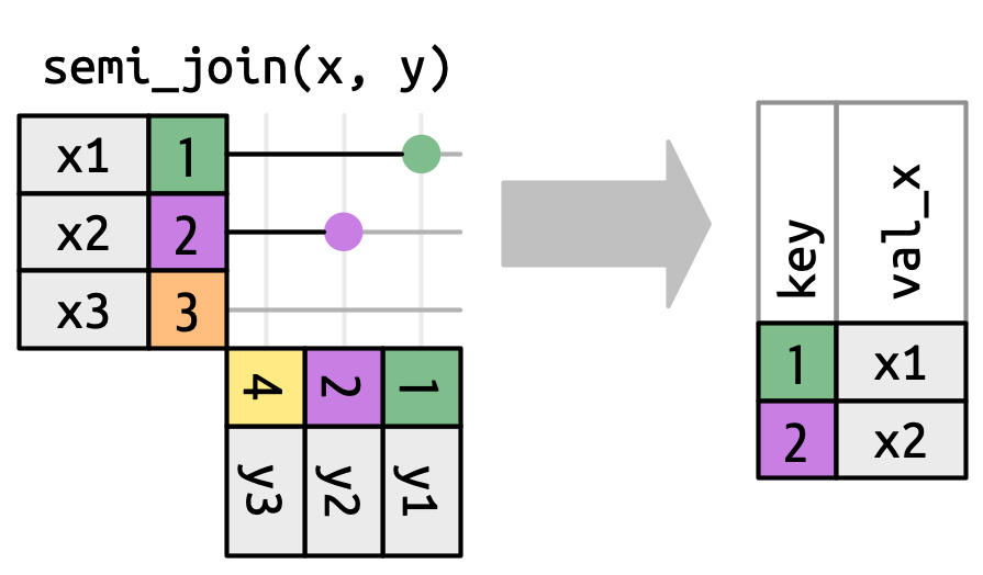
semi_join() keeps all the rows in primary that have a match in foreign. For example, the airports data set contains information on all airports in the US, but the flights data set only includes information on NYC airports. We can filter the airports data set to only include information on airports included in our foreign data frame (flights) using semi_join():
# A tibble: 3 × 8
  faa   name                  lat   lon   alt    tz dst   tzone
  <chr> <chr>               <dbl> <dbl> <dbl> <dbl> <chr> <chr>
1 EWR   Newark Liberty Intl  40.7 -74.2    18    -5 A     America/New_York
2 JFK   John F Kennedy Intl  40.6 -73.8    13    -5 A     America/New_York
3 LGA   La Guardia           40.8 -73.9    22    -5 A     America/New_York
Here is a visualization of this filtering process:
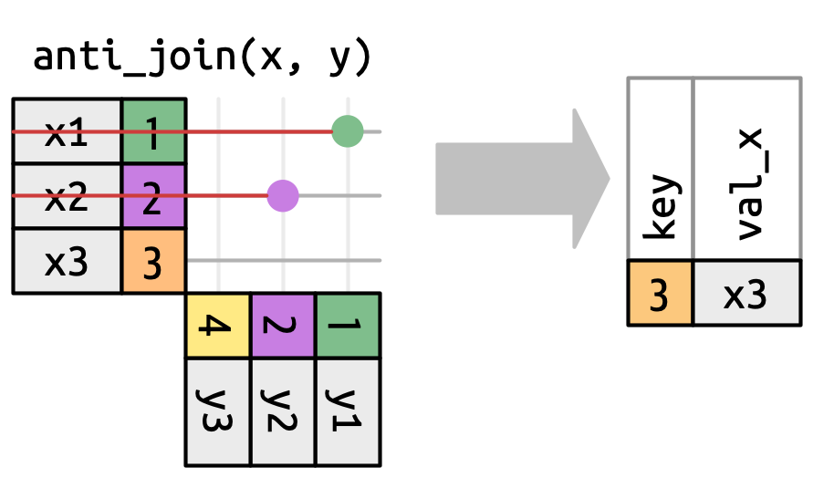
anti_join(), on the other hand, returns only the rows that do not have a match in foreign. For example, the following will return all airports except those included in the flights data frame:
# A tibble: 1,455 × 8
   faa   name                             lat    lon   alt    tz dst   tzone
   <chr> <chr>                          <dbl>  <dbl> <dbl> <dbl> <chr> <chr>
 1 04G   Lansdowne Airport               41.1  -80.6  1044    -5 A     America/…
 2 06A   Moton Field Municipal Airport   32.5  -85.7   264    -6 A     America/…
 3 06C   Schaumburg Regional             42.0  -88.1   801    -6 A     America/…
 4 06N   Randall Airport                 41.4  -74.4   523    -5 A     America/…
 5 09J   Jekyll Island Airport           31.1  -81.4    11    -5 A     America/…
 6 0A9   Elizabethton Municipal Airport  36.4  -82.2  1593    -5 A     America/…
 7 0G6   Williams County Airport         41.5  -84.5   730    -5 A     America/…
 8 0G7   Finger Lakes Regional Airport   42.9  -76.8   492    -5 A     America/…
 9 0P2   Shoestring Aviation Airfield    39.8  -76.6  1000    -5 U     America/…
10 0S9   Jefferson County Intl           48.1 -123.    108    -8 A     America/…
# ℹ 1,445 more rows
Here is a visualization of what is going on with anti_join():
Cross joins
Another common joining task includes finding all combinations of variables. For example, I often need to build data sets that include information on all countries across some number of years. I like to create this “spine” independently of my data collection to make sure I am covering all country-years I expect to cover and not relying on my data source.
For example, I may want to look at delays across all airports in the US in the years 2018-2024. To build my spine, I would start with a list of all airports:
airports# A tibble: 1,458 × 8
faa name lat lon alt tz dst tzone
<chr> <chr> <dbl> <dbl> <dbl> <dbl> <chr> <chr>
1 04G Lansdowne Airport 41.1 -80.6 1044 -5 A America/…
2 06A Moton Field Municipal Airport 32.5 -85.7 264 -6 A America/…
3 06C Schaumburg Regional 42.0 -88.1 801 -6 A America/…
4 06N Randall Airport 41.4 -74.4 523 -5 A America/…
5 09J Jekyll Island Airport 31.1 -81.4 11 -5 A America/…
6 0A9 Elizabethton Municipal Airport 36.4 -82.2 1593 -5 A America/…
7 0G6 Williams County Airport 41.5 -84.5 730 -5 A America/…
8 0G7 Finger Lakes Regional Airport 42.9 -76.8 492 -5 A America/…
9 0P2 Shoestring Aviation Airfield 39.8 -76.6 1000 -5 U America/…
10 0S9 Jefferson County Intl 48.1 -123. 108 -8 A America/…
# ℹ 1,448 more rowsNow, I want to create new rows for each airport and year between 2018 and 2024. For example, I want seven rows for Lansdowne Airport (Lansdowne Airport in 2018, Lansdowne Airport in 2019, etc.). To do this, I can use cross_join() to join airports to a new data frame I create with a row for each year in my scope:
airports |>
  cross_join(tibble(year = 2018:2024)) |>
  relocate(year)
# A tibble: 10,206 × 9
year faa name lat lon alt tz dst tzone
<int> <chr> <chr> <dbl> <dbl> <dbl> <dbl> <chr> <chr>
1 2018 04G Lansdowne Airport 41.1 -80.6 1044 -5 A Amer…
2 2019 04G Lansdowne Airport 41.1 -80.6 1044 -5 A Amer…
3 2020 04G Lansdowne Airport 41.1 -80.6 1044 -5 A Amer…
4 2021 04G Lansdowne Airport 41.1 -80.6 1044 -5 A Amer…
5 2022 04G Lansdowne Airport 41.1 -80.6 1044 -5 A Amer…
6 2023 04G Lansdowne Airport 41.1 -80.6 1044 -5 A Amer…
7 2024 04G Lansdowne Airport 41.1 -80.6 1044 -5 A Amer…
8 2018 06A Moton Field Municipal Airport 32.5 -85.7 264 -6 A Amer…
9 2019 06A Moton Field Municipal Airport 32.5 -85.7 264 -6 A Amer…
10 2020 06A Moton Field Municipal Airport 32.5 -85.7 264 -6 A Amer…
# ℹ 10,196 more rowsIf you have two vectors (not great, big data frames) that you want to find all combinations for, you can use crossing():
# A tibble: 10,206 × 2
    year faa
   <int> <chr>
 1  2018 04G
 2  2018 06A
 3  2018 06C
 4  2018 06N
 5  2018 09J
 6  2018 0A9
 7  2018 0G6
 8  2018 0G7
 9  2018 0P2
10  2018 0S9
# ℹ 10,196 more rows
Note
I will use crossing() to help build a 3D plot in the next part of this session: Estimating Causal Effects with Observational Data.