Session 2: Using Randomized Experiments to Estimate Causal Effects

Introduction

We often want to better understand what factors lead to (or cause) certain outcomes of interest. This session explains how we might go about identifying these causal effects in the real-world.

Our goal as political scientists is to explain whether (and why) changes to some features lead to changes in our outcomes of interest. For example:

Does increasing the number of voting booths close to a potential voter make that person more likely to vote?
Are peace treaties signed with a single, cohesive group more durable than those signed with many factionalized rebel groups?
Does trade between two countries make war between them less likely?

The questions can be reframed as causal statements that can then be tested:

More local voting booths lead to an increased likelihood individuals vote.
More factionalization among rebel groups leads to a higher likelihood the conflict will restart.
More trade between two countries leads to a lower likelihood that war will break out between them.

However, proving that changes to one factor (more local voting booths, factionalization, or trade) caused changes to our outcome of interest is very difficult to do. This is because we need to prove that all the other things that changed before our outcome of interest changed weren’t the ones really driving that outcome. How do we do this?

We will spend the whole course answering this question. This session, we are going to focus on experiments, which are often called the “gold-standard” of causal research. To guide us through this session, we are going to look at research conducted by Professor Susan Hyde.

Set up

To complete this session, you need to load in the following R packages:

Install packages

To install new R packages, run the following (excluding the packages you have already installed):

install.packages(c("tidyverse", "DT", "patchwork"))

library(tidyverse)
library(DT)
library(patchwork)

Are election monitors effective at reducing election-day fraud in new democracies?

Hyde was very interested in election fraud. She wanted to uncover what things the international community could do to prevent elections from being stolen. Interestingly for her, she completed her PhD during a time in which the prevalence of international election monitors exploded. There was a sharp increase in the number of elections held in new democracies globally that included international organizations or representatives from other countries monitoring how those elections were run. So, she wanted to know: did these international monitors cause less election-day fraud in democratic elections?

She worked out that, although fraud itself is very difficult to see, its outcome is not. (Effective) cheating parties receive a greater vote share than they would had they not cheated. So she set out to see whether international election monitors camped out at election booths decreased the vote share won by cheating parties at those booths. In her own words (Hyde 2007, 39):

If the presence of international observers causes a reduction in election-day fraud, the effect of observers should be visible at the subnational level by comparing polling stations that were visited by observers with those that were not visited. More specifically, if international monitoring reduces election day fraud directly, all else held equal, the cheating parties should gain less of their ill-gotten vote share in polling stations that were visited by international monitors.

So, Hyde offers the following sequence of causes:

International election monitors cause …
Less election-day fraud at the booth at which they are stationed (which we cannot observe directly), which causes …
A lower vote-share won by the cheating party than they would otherwise have won (which we can observe directly, kind of … stay tuned).

Causal relationships

Warning

Jargon incoming!

Hyde is interested in the causal relationship between international election monitors and election-day fraud. Formally, a causal relationship refers to the directional connection between a change in one variable and a corresponding change in another.

For causal relationships, direction really matters. You need to prove the following sequence of events:

A change happened to some factor, then:
A change happened to your outcome of interest

Let’s label these factors to avoid confusion. The treatment variable is the variable causing changes to another variable. It’s the one that moves first. The outcome variable is the variable changing as a result of changes to another variable (the treatment). It’s the one that moves second.

Hyde wanted to test whether the presence of international monitors (the treatment) leads to less election day fraud (the outcome).

Focus for a moment on the treatment variable. At any given polling station in any given election, monitors may be: 1) present, or 2) not present. We, therefore, have two conditions:

Treatment: monitors are present
Control: monitors are not present

Individual causal effects

We want to know whether the treatment causes a change in our outcome of interest. To do this, we want to compare the vote share the cheating party received at the voting booth with election monitors present (under treatment) to that it received at the voting booth without election monitors present (under control). Huh…

Let’s step through this with a concrete example. Imagine that we are looking at a specific election held within a new democracy. There are 1,000 election booths set up for the election.

In an ideal world, we would run the election with no monitors and record the vote share each party received at each booth. We would then jump in our very handy time machine and go back to the start of the election. We would station monitors at every booth, run the election, and record the vote share each party received.

We could then directly compare the vote share each party received at each booth with and without monitors (in treatment and control). If Hyde’s hypothesis is correct, we should see that the cheating party receives a lower vote share in the timeline with election monitors than it does in the timeline without them.

For example, imagine that the following results were recorded for the cheating party at each of the 1,000 booths in both timelines:

Because the only difference between these two versions of the election was the presence of election monitors, we can definitively state that the difference in vote shares won by each party was caused by the monitors. Let’s calculate those differences:

indiv_effect_df |> 
  mutate(across(vote_share_monitored:difference, 
                ~ scales::percent(.x, accuracy = 0.1))) |> 
  rename(ID = polling_station_id,
         `Monitored vote %` = vote_share_monitored,
         `Non-monitored vote %` = vote_share_not_monitored,
         Difference = difference) |> 
  datatable(rownames = F, options = list(pageLength = 10, dom = 'tip'))

In this hypothetical election, these differences are substantial! They are often the difference between a decisive victory and an embarrassing defeat.

Average causal effects

Sadly for us, however, we are yet to invent time machines. We cannot observe both the treatment and control for each individual booth. Rather what we see is the following:

We are, essentially, missing data for the counter-factual for each booth. We cannot, therefore, calculate the difference and identify the causal effect of election monitors for each individual booth. So, now what?

We need to move away from looking at individual booths and start to look for patterns in our group of observations. Let’s return to our two timelines. What was the difference between the vote share won by the cheating party with and without election monitors on average across all booths?

Avg. monitored vote %	Avg. non-monitored vote %	Difference
39.5%	84.3%	-44.8%

Okay, what is the difference, on average, in our real world?

Avg. monitored vote %	Avg. non-monitored vote %	Difference
40.2%	84.5%	-44.3%

The average difference with missing counter-factuals is very close to that with full information (that relies on that handy time machine). How does this work so well?

Skipping very far ahead…

In fact, if we ran many, many identical experiments – assigning monitors to booths randomly – and recorded the average difference in vote shares won in each of those many trials, the average of those averages would be the same as that found in our impossible world with full information. This is because of two important facts that are described as the Law of Large Numbers and the Central Limit Theorem. We will discuss these (and demonstrate them using simulations) in a couple of sessions’ time.

Randomization

Through randomization! I assigned monitors to the 1,000 voting booths randomly. For each booth, I flipped a (R generated) coin to decide whether that booth would be monitored. At the end of that process, roughly half of the booths had monitors and half did not:

Monitored	No. of booths
No	502
Yes	498

The magic trick with random assignment is that you tend to end up with two groups that are roughly identical to one another prior to treatment, on average. Remember, our goal is to create two groups (treatment and control) that are identical to one another prior to treatment. If the only difference between the groups is the treatment, we can say that any differences in our outcome of interest is caused by the treatment.

Absent a time machine, we then need to set about creating two groups that are as identical to each other as possible. It turns out that random assignment does a very good job of achieving this.

Note

Practitioners have come up with other clever ways of doing this, including pairwise matching. We will not cover those in this course.

You don’t need to take my word for this. Let’s prove it with simulation! Imagine we have a group of 1,000 individuals. We know the following about them:

Height
Weight
Eye colour

Here are those data:

I’m now going to flip a (imaginary, R-generated) coin for each of these 1,000 individuals to assigned them to either group A or B:

Now we can check how similar these two groups are to one another. Let’s start with their heights:

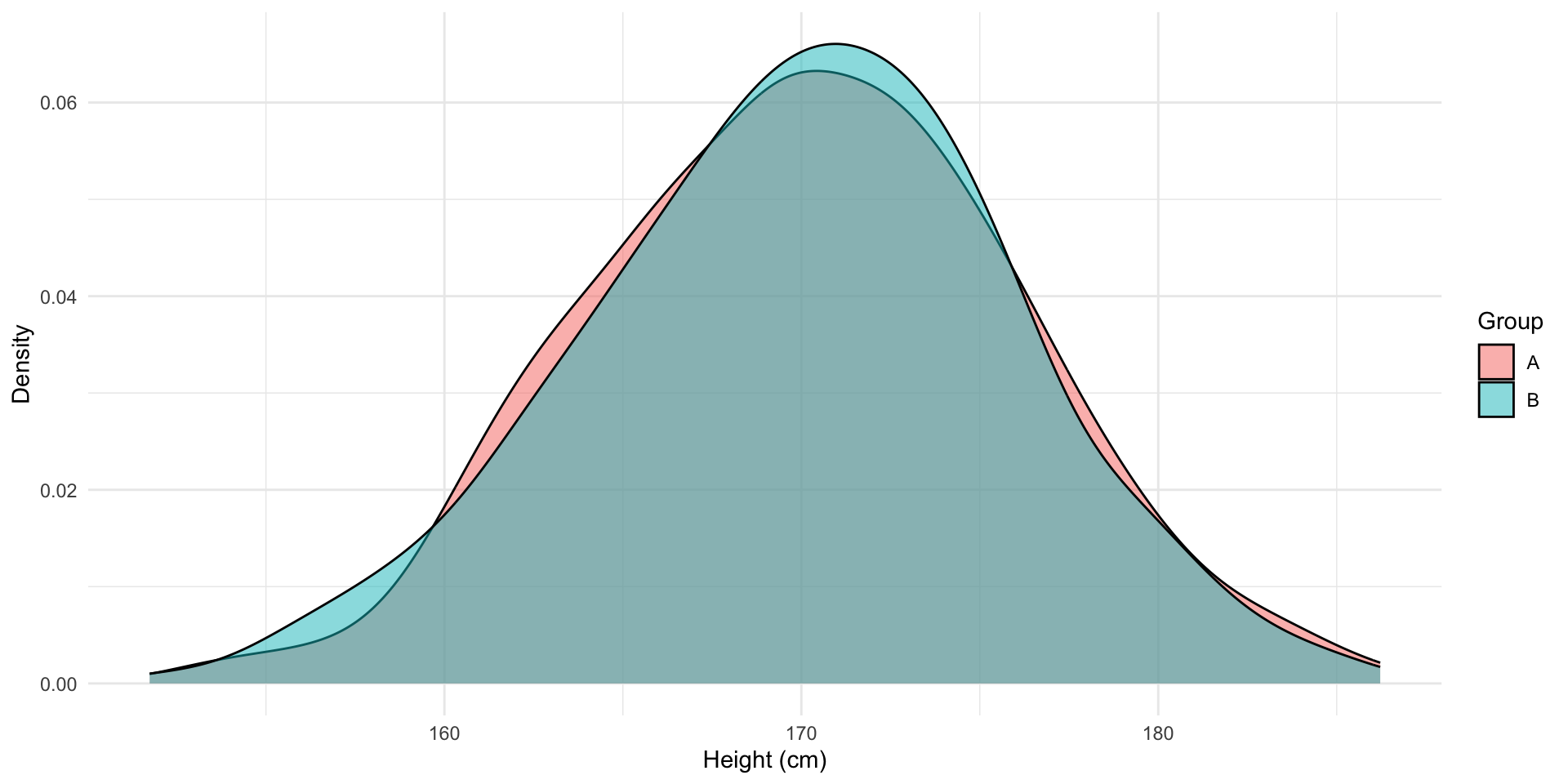
The distribution of heights among individuals in groups A and B are roughly identical. The average height of individuals in group A is 170.1 cm and in group B is 170 cm. Pretty neat!

Let’s check their weight:

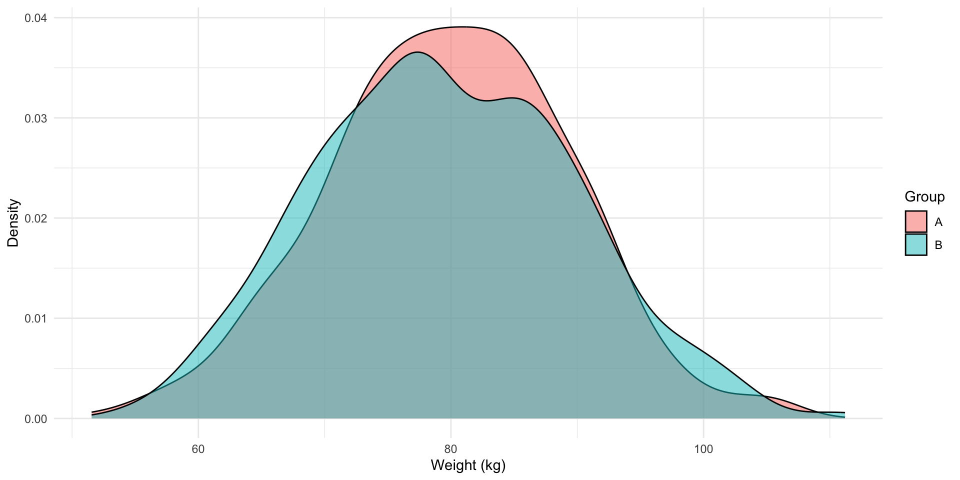
Similarly, the distribution of weights among individuals in groups A and B are roughly identical. On average, individuals in group A weigh 79.9 kg. Individuals in group B weigh 79.6 kg, on average.

Finally, let’s look at eye colour:

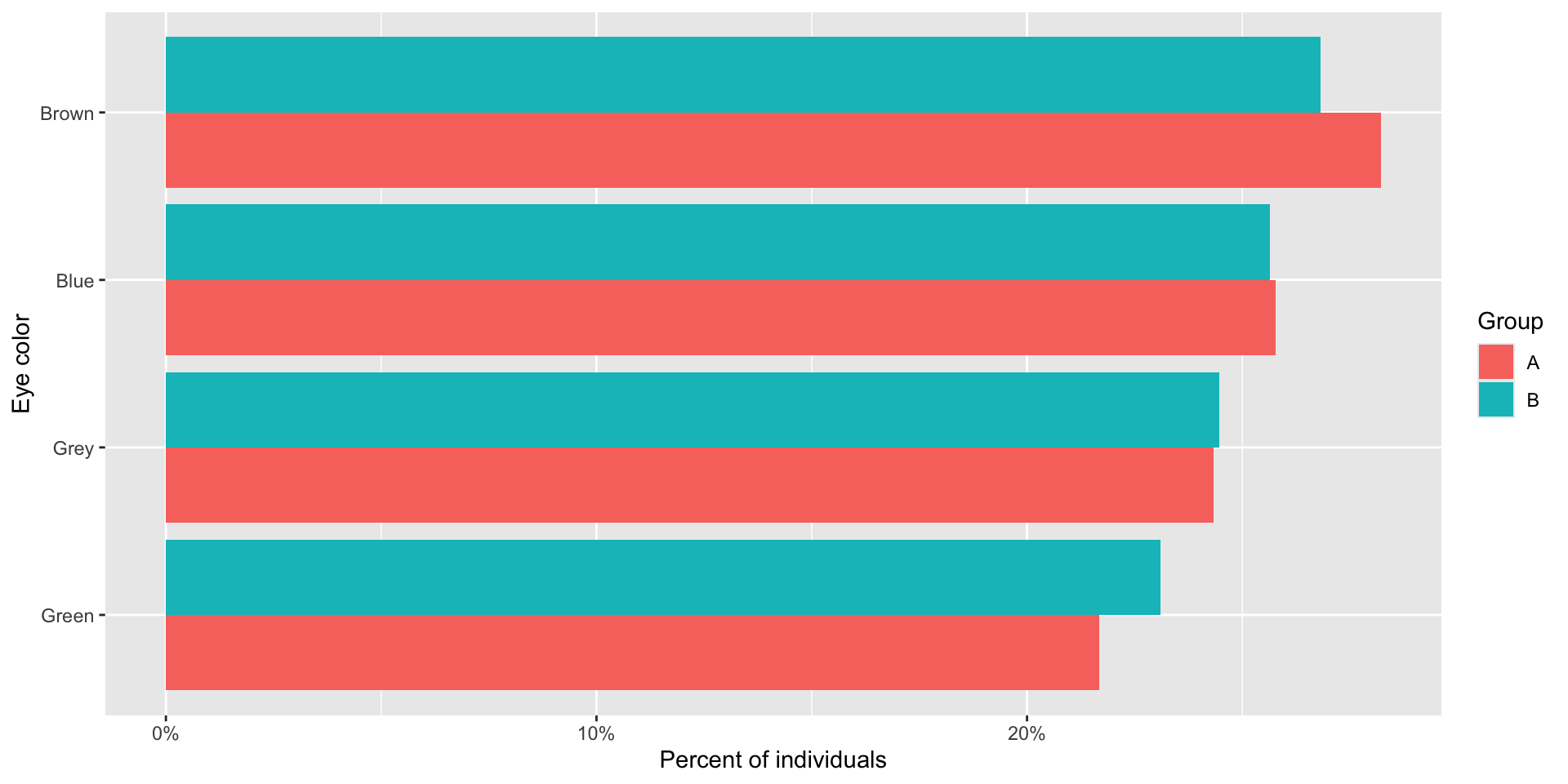
Again, the proportion of individuals within each group with each eye colour are roughly identical. This is all due to random assignment.

Let’s repeat this process, assigning our 1,000 individuals randomly to each group, and make sure this wasn’t a fluke:

And let’s see how similar these new, randomly-assigned groups are to each other:

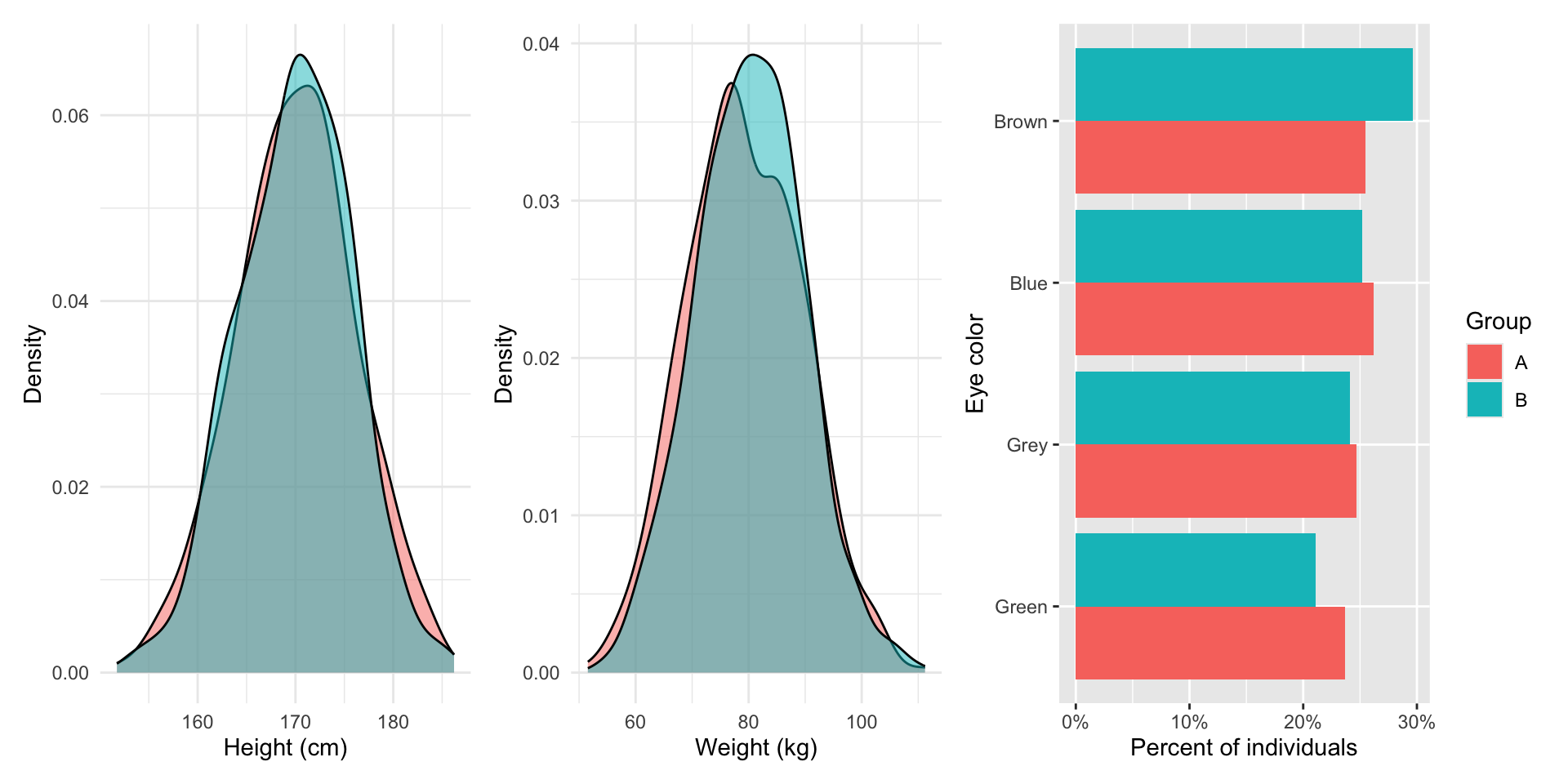
Again, these two groups are nearly identical to one another, on average.

Returning to our question

So, do international election monitors deter election-fraud? Yes! The international community monitored the 2003 Armenian Presidential elections. Monitors were assigned randomly to the polling stations. Hyde found a large difference between the vote share received by the cheating party at monitored stations compared to non-monitored stations, on average. She concluded that election monitors stationed at election booths reduced the amount of fraud committed at those booths.

She provides the following table in on page 53 of her paper:

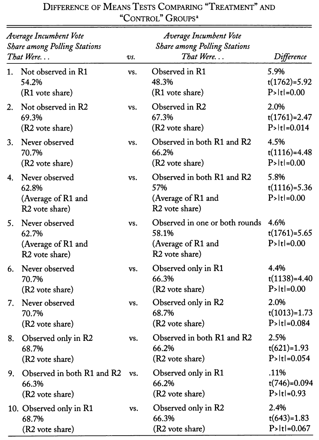
The vote proceeded in two rounds (demarcated R1 and R2 respectively). For now, focus on the percentage differences reported in the third column (we will get to all of those measures of uncertainty later in the course).

Let’s step through the first row together. Monitors were assigned randomly to election booths. Among the booths that were not observed in round one, the incumbent received 54.2% of the vote. Among the booths that were monitored, however, the incumbent only received 48.3% of the vote. This is a difference of a whopping 5.9% of the total vote share in round one.

Remember, monitors were assigned to booths randomly. Yes, these booths would be different from each other. Some would sit in electorates in which the incumbent would enjoy strong support and others would be in electorates in which they did not. Some would be in rural settings, whilst others would be in the center of town. However, because of the random assignment, these two groups of booths are probably very similar to one another on average. This allows Hyde to claim that the only meaningful difference between them was the treatment (presence of monitors). This, in turn, allows her to claim that the difference in vote share won (5.9%) was caused by the monitors.

This is a big difference! Elections can be won or lost by much smaller margins. It appears that monitors make a substantive difference to the vote share won. Hyde proved this all by simply looking at the difference between the averages of her two (randomly assigned) groups. This is excellent science: it is simple and clear.

We don’t often have the luxury of random assignment when attempting to answer political questions. Next we will explore how we can learn about general relationships between our variables of interest when we have incomplete information.

Quiz

Head over to ELMs to complete this session’s quiz. You need to score 80% on it to gain access to the next session’s quiz.

References

Hyde, Susan D. 2007. “The Observer Effect in International Politics: Evidence from a Natural Experiment.” World Politics 60 (1): 37–63. http://www.jstor.org/stable/40060180.