Registered S3 method overwritten by 'gdata':
  method         from
  reorder.factor gplots

Attaching package: 'poliscidata'

The following object is masked from 'package:infer':

    gss
The lecture first reviewed testing hypotheses about means and proportions before moving to the \(\chi^2\) test. We will follow that order here.
Hypothesis Testing for Means and Proportions
Much of political science research involves continuous variables (like income or ideological scores) or binary outcomes (like voting/not voting). The t-tests and proportion tests are our primary tools for these scenarios. We’ll use the GSS dataset for these examples.
One-Sample t-test: Testing a Single Mean
The one-sample t-test is used to test a specific prediction (\(H_a\)) about the value of a population mean (\(\mu\)) against the null hypothesis (\(H_0\)), which states the mean is equal to a null value (\(\mu_0\)).
Hypothesis Example: Is the average number of children for Americans surveyed in the GSS greater than \(2\)?
\(H_a: \mu < 2\)
\(H_0: \mu = 2\)
We use the children variable and the t.test() function, setting the hypothesized mean with mu and the directional hypothesis with alternative = “less”.
# 1. Prepare data (clean NAs)gss_children <- poliscidata::gss |>select(id, children = childs) |>drop_na()# 2. Calculate the meanmean(gss_children$children)
    One Sample t-test

data:  gss_children$children
t = -2.8651, df = 1970, p-value = 0.002106
alternative hypothesis: true mean is less than 2
95 percent confidence interval:
     -Inf 1.954003
sample estimates:
mean of x
 1.891933
If the p-value is small (e.g., \(< 0.05\)), we reject the null hypothesis, concluding that the true mean is indeed greater than 2.
Two-Sample t-test: Comparing Two Means
The two-sample t-test determines whether there is a statistically significant difference between the means of two independent groups. The null hypothesis is always that there is no difference between the two means.
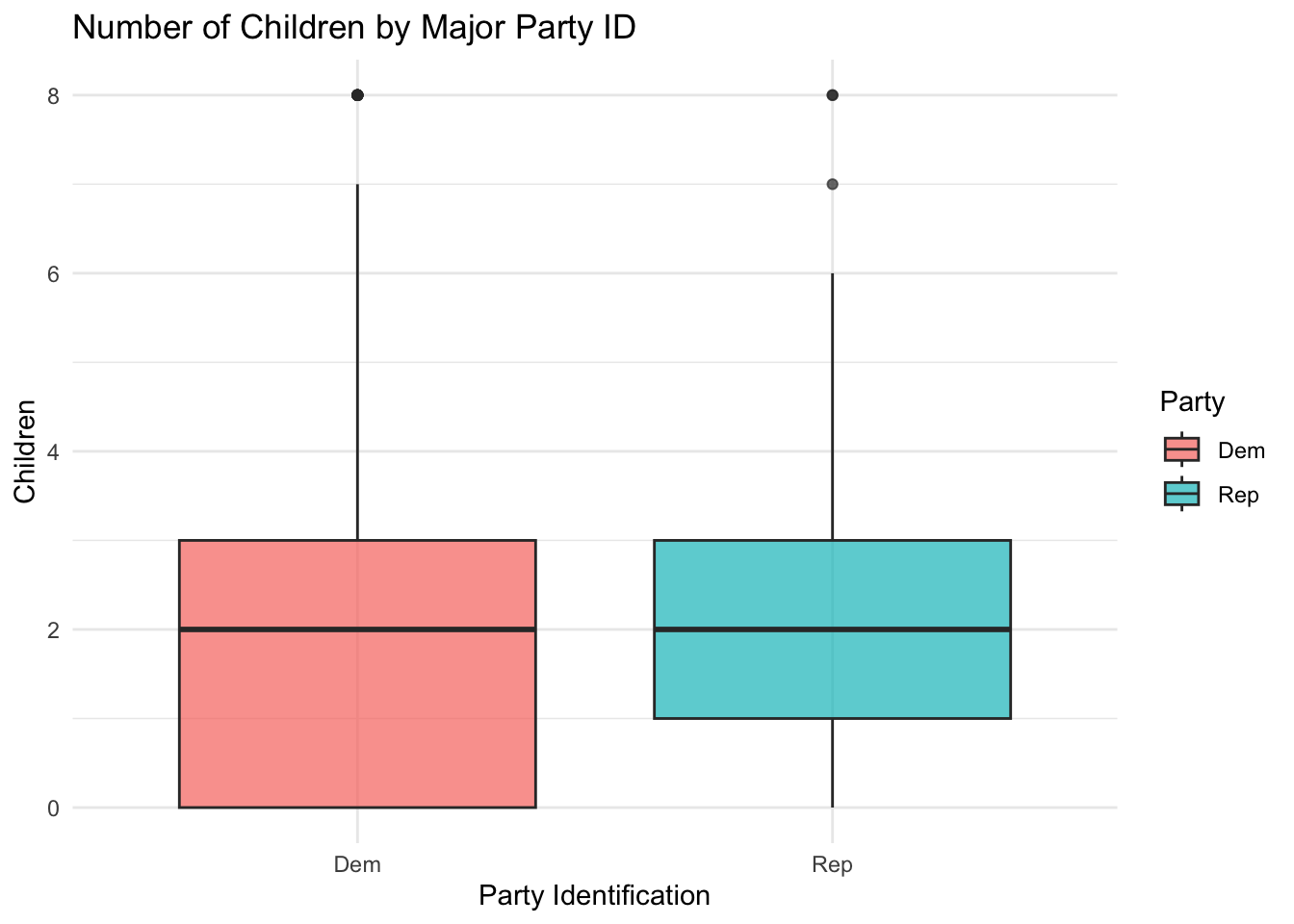
Hypothesis Example: Do Democrats have a smaller average number of children than Republicans?
We’ll use partyid_3 (Democrat vs. Republican) and children.
# 1. Filter the data for only Democrats and Republicansgss_child_party <- poliscidata::gss |>filter(partyid_3 %in%c("Dem", "Rep")) |>select(childs, partyid_3) |>drop_na()# 2. Visualize the income distribution by partygss_child_party |>ggplot(aes(x = partyid_3, y = childs, fill = partyid_3)) +geom_boxplot(alpha =0.7) +labs(title ="Number of Children by Major Party ID",x ="Party Identification",y ="Children",fill ="Party") +theme_minimal()
We run the two-sample test using the formula interface DV ~ IV.
# 3. Perform the two-sample t-test (comparing Republican vs. Democrat means)two_sample_t_test <-t.test(childs ~ partyid_3,data = gss_child_party,# Testing if Democrat's mean is greateralternative ="less",var.equal = T) two_sample_t_test
    Two Sample t-test

data:  childs by partyid_3
t = -1.1835, df = 1138, p-value = 0.1184
alternative hypothesis: true difference in means between group Dem and group Rep is less than 0
95 percent confidence interval:
       -Inf 0.04604209
sample estimates:
mean in group Dem mean in group Rep
         1.816619          1.934389
One-Sample Proportion Test: Testing a Single Proportion
This test is used for a specific prediction about a proportion (\(\pi\)) in a population, often when dealing with binary outcomes (e.g., support/oppose, vote/don’t vote).
Hypothesis Example: We hypothesize that the proportion of people who believe the federal government is spending too little on the environment is greater than 50% (\(\pi_0 = 0.5\)).
\(H_a: \pi > 0.5\)
\(H_0: \pi = 0.5\)
We use the natenvir variable, convert it into a binary outcome, and use prop.test().
# 1. Prepare the data: create a binary variable for "Too little"gss_envir <- poliscidata::gss |>select(natenvir) |>drop_na() |>mutate(is_too_little =ifelse(natenvir =="Too little", 1, 0) )# 2. Calculate the total successes (x) and sample size (n)x_successes <-sum(gss_envir$is_too_little)n_obs <-nrow(gss_envir)# 3. Use prop.test() for the one-sample proportion testprop_test_one_sample <-prop.test(x = x_successes,n = n_obs,p =0.5, # Null hypothesized proportionalternative ="greater")prop_test_one_sample
    1-sample proportions test with continuity correction

data:  x_successes out of n_obs, null probability 0.5
X-squared = 21.953, df = 1, p-value = 1.397e-06
alternative hypothesis: true p is greater than 0.5
95 percent confidence interval:
 0.5489139 1.0000000
sample estimates:
        p
0.5756952
Two-Sample Proportion Test: Comparing Two Proportions
This test compares the proportions of “success” between two independent groups.
Hypothesis Example: Is the proportion of Democrats who believe the government is spending too little on the environment higher than the proportion of Republicans?
# 1. Filter and summarize successes/totals for the two groupsgss_envir_party_summary <- poliscidata::gss |>filter(partyid_3 %in%c("Dem", "Rep")) |>select(natenvir, partyid_3) |>drop_na() |>mutate(is_too_little =ifelse(natenvir =="Too little", 1, 0) ) |>group_by(partyid_3) |>summarise(successes =sum(is_too_little),n =n() ) |>ungroup()# 2. Extract the counts of successes and sample sizes in the required formatx_counts <- gss_envir_party_summary$successesn_samples <- gss_envir_party_summary$n# 3. Use prop.test() for the two-sample proportion testprop_test_two_sample <-prop.test(x = x_counts, # Vector of successesn = n_samples, # Vector of total sample sizesalternative ="greater")prop_test_two_sample
    2-sample test for equality of proportions with continuity correction

data:  x_counts out of n_samples
X-squared = 47.319, df = 1, p-value = 3.016e-12
alternative hypothesis: greater
95 percent confidence interval:
 0.2283152 1.0000000
sample estimates:
   prop 1    prop 2
0.6824513 0.3816425
Chi-Square Test for Independence (Two-Way Tables)
The second part of the lecture focused on the \(\chi^2\) test, which is used when we want to test for a relationship (independence) between two categorical variables.
Federal spending on parks and recreation
We will explore hypothesis testing across categorical variables by answering the question: is an individual’s party identification associated with their support for current levels of federal spending on parks and recreation? We will use data from the GSS, obtained using poliscidata::gss.
\(H_a\): Party identification and support for federal park spending are associated (dependent).
\(H_0\): Party identification and support for federal park spending are independent.
gss <- poliscidata::gss |># Select only the relevant columnsselect(id, partyid_3, natpark) |># Remove non-complete responsesdrop_na()
Calculating our observed counts
First, we need to look at our observed data. We will make a cross tab of the data using modelsummary::datasummary_crosstab().
datasummary_crosstab(natpark ~ partyid_3, data = gss,statistic =1~1+ N +Percent("col"))
natpark
Dem
Ind
Rep
All
Too little
N
239
251
104
594
% col
35.1
33.6
24.2
32.0
About right
N
413
450
290
1153
% col
60.7
60.2
67.6
62.1
Too much
N
28
46
35
109
% col
4.1
6.2
8.2
5.9
All
N
680
747
429
1856
% col
100.0
100.0
100.0
100.0
The GSS surveyed 1,856 individuals in 2012, asking them of their party identification and level of support for current federal spending on parks and recreation.
Calculating our expected counts
If the null hypothesis were true—that is, if party identification and support for federal park spending are independent—then the counts in each cell would reflect the overall row and column marginal probabilities.
To find the expected count for any given cell, we use the formula:
    Pearson's Chi-squared test

data:  gss$natpark and gss$partyid_3
X-squared = 20.964, df = 4, p-value = 0.000322
Since the p-value is extremely small, we reject the null hypothesis and conclude that there is a statistically significant association between party identification and support for federal park spending.
Concluding Summary
This lab has walked us through the full range of common hypothesis tests you’ll use in political science:
t-tests for comparing means of continuous variables.
Proportion tests for comparing proportions of binary variables.
Chi-squared tests for exploring the association between two categorical variables.
You are now equipped with the R skills to put the lecture’s theoretical concepts into practice. Remember, the core logic is the same across all these tests: Assume \(H_0\) is true, calculate a test statistic, and see how likely that statistic is to occur under the null distribution.