Data Transformation

Set up

To complete this session, you need to load in the following R packages:

Install packages

To install new R packages, run the following (excluding the packages you have already installed):

install.packages("gapminder")

library(tidyverse)
library(gapminder)

This section focuses on introducing you to some new R skills. Data rarely come to us perfectly formatted and without annoying errors or inconsistencies. We can use R to clean our data up and get them ready for analysis.

Gapminder

This session, we will explore the long-studied relationship between countries’ health and wealth. Attention was brought to this relationship by the Gapminder project. You can read more about their research here.

Before we get started, check out this video that describes (very enthusiastically) the relationship between health and wealth:

Introduction

Today, I am going to introduce you to some of my most widely used functions in R. The dplyr R package, which houses these functions, focuses on providing you with some very helpful tools to tidy your data. This step in the data analysis process is critical, and often one of the most time consuming, so let’s get started!

R objects

As a reminder, objects sit in R’s memory. You can see which ones exist in your current session and their values over in the environment tab.

To create a new object, use: <-. You can update that object at any time.

Note

Some people use = instead of <-. I strongly recommend against this. It makes your script difficult to read, and it can lead to syntax errors.

R functions

Functions are helpful short-hands that perform specific tasks in R. Many of these functions come straight out of the box with R. For example, you can run the following code without loading any packages into your current session:

seq(1, 10)

 [1]  1  2  3  4  5  6  7  8  9 10

Tip

The seq() function takes three main arguments: a start value, end value, and interval value. Above I have asked it to start at 1 and end at 10. By default, its interval value is 1. Therefore, its output is every whole number from 1 to 10.

You can even create objects with R functions:

x <- seq(1, 10)

x

 [1]  1  2  3  4  5  6  7  8  9 10

Now, the x object is a vector of all 10 whole numbers from 1 to 10.

Data

As mentioned above, we are going to be using the Gapminder project’s data on countries’ health and wealth to explore data transformation. Happily, there is an R package that provides that data for us. We will now install it:

install.packages("gapminder")

Next, you want to create a new script for this session. At the top of that script, include the code to load in the packages we will be using today:

library(tidyverse)
library(gapminder)

You can now access the Gapminder data directly:

gapminder

# A tibble: 1,704 × 6
   country     continent  year lifeExp      pop gdpPercap
   <fct>       <fct>     <int>   <dbl>    <int>     <dbl>
 1 Afghanistan Asia       1952    28.8  8425333      779.
 2 Afghanistan Asia       1957    30.3  9240934      821.
 3 Afghanistan Asia       1962    32.0 10267083      853.
 4 Afghanistan Asia       1967    34.0 11537966      836.
 5 Afghanistan Asia       1972    36.1 13079460      740.
 6 Afghanistan Asia       1977    38.4 14880372      786.
 7 Afghanistan Asia       1982    39.9 12881816      978.
 8 Afghanistan Asia       1987    40.8 13867957      852.
 9 Afghanistan Asia       1992    41.7 16317921      649.
10 Afghanistan Asia       1997    41.8 22227415      635.
# ℹ 1,694 more rows

Above, R prints out some useful information about our data. First, we learn that it is a tibble. This is the tidyverse version of a data frame.

Second, we learn how many rows and columns are included in our data set. We have 1,704 rows and 6 columns.

Next, we learn the column (or variable) titles:

colnames(gapminder)

[1] "country"   "continent" "year"      "lifeExp"   "pop"       "gdpPercap"

Next, we see some funny looking three letter words under each column name. These refer to the column’s data type. We will discuss these below.

Finally, we see the first few rows of our data set. We can see that each row provides a country’s information in a single year.

Data types

Those funny three-letter words refer to the column’s data type. In this data set, we have three different types:

• <fct>, which stands for factor (R’s word for categorical variable)

• <int>, which stands for integer

• <dbl>, which stands for double (or real number)

Some other common data types include:

• <chr>, which stands for character (or string)

• <dttm>, which stands for date-time

• <lgl>, which stands for local (which can only be TRUE or FALSE)

Data types are important because each column can only contain one data type. You cannot, for example, include a character in an integer column (imagine trying to run some calculation on that column: how would R treat the stray character value?).

dplyr basics

Now we know a little bit more about our data set, we are going to use it to explore five of the most commonly used functions in R:

• filter()

• arrange()

• select()

• mutate()

• summarise()

Exercises

What is the unit of observation for the gapminder data set?

Check your answer

The unit of observation is country-year.

How many country-years are included in the gapminder data set?

Check your answer

nrow(gapminder)

[1] 1704

Which two variables in the gapminder data set are factors?

Check your answer

country and continent are factors (or categorical variables).

Filtering your data

We are going to start by learning how to filter our data to only include those observations we are interested in exploring.

All dplyr functions are structured the same way. They take the data object you want to transform as their first argument. You then need to identify the columns within that data object you want to transform and what you want to do with them.

For example, the following code takes our data set, gapminder, and tells filter() that we want to only include rows in which the country column matches “Australia” and the year column is greater than 2000:

filter(gapminder, country == "Australia", year > 2000)

# A tibble: 2 × 6
  country   continent  year lifeExp      pop gdpPercap
  <fct>     <fct>     <int>   <dbl>    <int>     <dbl>
1 Australia Oceania    2002    80.4 19546792    30688.
2 Australia Oceania    2007    81.2 20434176    34435.

We can ask filter() to include rows that match multiple values:

filter(gapminder, continent %in% c("Asia", "Oceania"))

# A tibble: 420 × 6
   country     continent  year lifeExp      pop gdpPercap
   <fct>       <fct>     <int>   <dbl>    <int>     <dbl>
 1 Afghanistan Asia       1952    28.8  8425333      779.
 2 Afghanistan Asia       1957    30.3  9240934      821.
 3 Afghanistan Asia       1962    32.0 10267083      853.
 4 Afghanistan Asia       1967    34.0 11537966      836.
 5 Afghanistan Asia       1972    36.1 13079460      740.
 6 Afghanistan Asia       1977    38.4 14880372      786.
 7 Afghanistan Asia       1982    39.9 12881816      978.
 8 Afghanistan Asia       1987    40.8 13867957      852.
 9 Afghanistan Asia       1992    41.7 16317921      649.
10 Afghanistan Asia       1997    41.8 22227415      635.
# ℹ 410 more rows

Here, I have used the %in% value and a vector (which is c(...)) of strings to ask filter to include all rows in which the continent column matches the values “Asia” and “Oceania”.

We can ask filter() to include values within a range. The following code asks filter() to include all rows in which the pop column is greater than 500,000 and less than 1,000,000:

filter(gapminder, pop > 500000 & pop < 1000000)

# A tibble: 88 × 6
   country  continent  year lifeExp    pop gdpPercap
   <fct>    <fct>     <int>   <dbl>  <int>     <dbl>
 1 Bahrain  Asia       1992    72.6 529491    19036.
 2 Bahrain  Asia       1997    73.9 598561    20292.
 3 Bahrain  Asia       2002    74.8 656397    23404.
 4 Bahrain  Asia       2007    75.6 708573    29796.
 5 Botswana Africa     1962    51.5 512764      984.
 6 Botswana Africa     1967    53.3 553541     1215.
 7 Botswana Africa     1972    56.0 619351     2264.
 8 Botswana Africa     1977    59.3 781472     3215.
 9 Botswana Africa     1982    61.5 970347     4551.
10 Comoros  Africa     1997    60.7 527982     1174.
# ℹ 78 more rows

The following code asks filter() to include all rows in which the pop column is greater than 500,000 or less than 1,000,000.

filter(gapminder, pop > 500000 | pop < 1000000)

# A tibble: 1,704 × 6
   country     continent  year lifeExp      pop gdpPercap
   <fct>       <fct>     <int>   <dbl>    <int>     <dbl>
 1 Afghanistan Asia       1952    28.8  8425333      779.
 2 Afghanistan Asia       1957    30.3  9240934      821.
 3 Afghanistan Asia       1962    32.0 10267083      853.
 4 Afghanistan Asia       1967    34.0 11537966      836.
 5 Afghanistan Asia       1972    36.1 13079460      740.
 6 Afghanistan Asia       1977    38.4 14880372      786.
 7 Afghanistan Asia       1982    39.9 12881816      978.
 8 Afghanistan Asia       1987    40.8 13867957      852.
 9 Afghanistan Asia       1992    41.7 16317921      649.
10 Afghanistan Asia       1997    41.8 22227415      635.
# ℹ 1,694 more rows

R includes some handy operators:

• == is equal to

• != is not equal to

• >= is greater than or equal to

• <= is less than or equal to

• | is OR

• & is AND

• %in% is in

Exercises

Find all country-years that have populations greater than 1 billion people.

Check your answer

filter(gapminder, pop > 1e9)

# A tibble: 8 × 6
  country continent  year lifeExp        pop gdpPercap
  <fct>   <fct>     <int>   <dbl>      <int>     <dbl>
1 China   Asia       1982    65.5 1000281000      962.
2 China   Asia       1987    67.3 1084035000     1379.
3 China   Asia       1992    68.7 1164970000     1656.
4 China   Asia       1997    70.4 1230075000     2289.
5 China   Asia       2002    72.0 1280400000     3119.
6 China   Asia       2007    73.0 1318683096     4959.
7 India   Asia       2002    62.9 1034172547     1747.
8 India   Asia       2007    64.7 1110396331     2452.

Note: 1e9 is scientific notation for 1 billion (which has nine zeros).

Find all countries in Oceania.

Check your answer

filter(gapminder, continent == "Oceania")

# A tibble: 24 × 6
   country   continent  year lifeExp      pop gdpPercap
   <fct>     <fct>     <int>   <dbl>    <int>     <dbl>
 1 Australia Oceania    1952    69.1  8691212    10040.
 2 Australia Oceania    1957    70.3  9712569    10950.
 3 Australia Oceania    1962    70.9 10794968    12217.
 4 Australia Oceania    1967    71.1 11872264    14526.
 5 Australia Oceania    1972    71.9 13177000    16789.
 6 Australia Oceania    1977    73.5 14074100    18334.
 7 Australia Oceania    1982    74.7 15184200    19477.
 8 Australia Oceania    1987    76.3 16257249    21889.
 9 Australia Oceania    1992    77.6 17481977    23425.
10 Australia Oceania    1997    78.8 18565243    26998.
# ℹ 14 more rows

Find all countries in both Asia and Europe.

Check your answer

filter(gapminder, continent %in% c("Asia", "Europe"))

# A tibble: 756 × 6
   country     continent  year lifeExp      pop gdpPercap
   <fct>       <fct>     <int>   <dbl>    <int>     <dbl>
 1 Afghanistan Asia       1952    28.8  8425333      779.
 2 Afghanistan Asia       1957    30.3  9240934      821.
 3 Afghanistan Asia       1962    32.0 10267083      853.
 4 Afghanistan Asia       1967    34.0 11537966      836.
 5 Afghanistan Asia       1972    36.1 13079460      740.
 6 Afghanistan Asia       1977    38.4 14880372      786.
 7 Afghanistan Asia       1982    39.9 12881816      978.
 8 Afghanistan Asia       1987    40.8 13867957      852.
 9 Afghanistan Asia       1992    41.7 16317921      649.
10 Afghanistan Asia       1997    41.8 22227415      635.
# ℹ 746 more rows

Find all country-years that have a life expectancy greater than 50 years and less than 60 years.

Check your answer

filter(gapminder, lifeExp > 50 & lifeExp < 60)

# A tibble: 336 × 6
   country    continent  year lifeExp      pop gdpPercap
   <fct>      <fct>     <int>   <dbl>    <int>     <dbl>
 1 Albania    Europe     1952    55.2  1282697     1601.
 2 Albania    Europe     1957    59.3  1476505     1942.
 3 Algeria    Africa     1967    51.4 12760499     3247.
 4 Algeria    Africa     1972    54.5 14760787     4183.
 5 Algeria    Africa     1977    58.0 17152804     4910.
 6 Bahrain    Asia       1952    50.9   120447     9867.
 7 Bahrain    Asia       1957    53.8   138655    11636.
 8 Bahrain    Asia       1962    56.9   171863    12753.
 9 Bahrain    Asia       1967    59.9   202182    14805.
10 Bangladesh Asia       1982    50.0 93074406      677.
# ℹ 326 more rows

Find all country-years that have a life expectancy less than 50 years or greater than 60 years.

Check your answer

filter(gapminder, lifeExp < 50 | lifeExp > 60)

# A tibble: 1,368 × 6
   country     continent  year lifeExp      pop gdpPercap
   <fct>       <fct>     <int>   <dbl>    <int>     <dbl>
 1 Afghanistan Asia       1952    28.8  8425333      779.
 2 Afghanistan Asia       1957    30.3  9240934      821.
 3 Afghanistan Asia       1962    32.0 10267083      853.
 4 Afghanistan Asia       1967    34.0 11537966      836.
 5 Afghanistan Asia       1972    36.1 13079460      740.
 6 Afghanistan Asia       1977    38.4 14880372      786.
 7 Afghanistan Asia       1982    39.9 12881816      978.
 8 Afghanistan Asia       1987    40.8 13867957      852.
 9 Afghanistan Asia       1992    41.7 16317921      649.
10 Afghanistan Asia       1997    41.8 22227415      635.
# ℹ 1,358 more rows

Sorting your data

We can control the order of our data using arrange(). The following code sorts our data by country name (alphabetically) and year (in ascending numerical order):

arrange(gapminder, country, year)

# A tibble: 1,704 × 6
   country     continent  year lifeExp      pop gdpPercap
   <fct>       <fct>     <int>   <dbl>    <int>     <dbl>
 1 Afghanistan Asia       1952    28.8  8425333      779.
 2 Afghanistan Asia       1957    30.3  9240934      821.
 3 Afghanistan Asia       1962    32.0 10267083      853.
 4 Afghanistan Asia       1967    34.0 11537966      836.
 5 Afghanistan Asia       1972    36.1 13079460      740.
 6 Afghanistan Asia       1977    38.4 14880372      786.
 7 Afghanistan Asia       1982    39.9 12881816      978.
 8 Afghanistan Asia       1987    40.8 13867957      852.
 9 Afghanistan Asia       1992    41.7 16317921      649.
10 Afghanistan Asia       1997    41.8 22227415      635.
# ℹ 1,694 more rows

To sort in descending order, simply wrap your column name in the desc() function:

arrange(gapminder, country, desc(year))

# A tibble: 1,704 × 6
   country     continent  year lifeExp      pop gdpPercap
   <fct>       <fct>     <int>   <dbl>    <int>     <dbl>
 1 Afghanistan Asia       2007    43.8 31889923      975.
 2 Afghanistan Asia       2002    42.1 25268405      727.
 3 Afghanistan Asia       1997    41.8 22227415      635.
 4 Afghanistan Asia       1992    41.7 16317921      649.
 5 Afghanistan Asia       1987    40.8 13867957      852.
 6 Afghanistan Asia       1982    39.9 12881816      978.
 7 Afghanistan Asia       1977    38.4 14880372      786.
 8 Afghanistan Asia       1972    36.1 13079460      740.
 9 Afghanistan Asia       1967    34.0 11537966      836.
10 Afghanistan Asia       1962    32.0 10267083      853.
# ℹ 1,694 more rows

You can combine arrange() and filter() using the slice_X() functions. For example, you can filter for the smallest value in a column using slice_min(). The following code filters for the smallest value in the lifeExp column:

slice_min(gapminder, lifeExp)

# A tibble: 1 × 6
  country continent  year lifeExp     pop gdpPercap
  <fct>   <fct>     <int>   <dbl>   <int>     <dbl>
1 Rwanda  Africa     1992    23.6 7290203      737.

The following code filters for the largest value in this column:

slice_max(gapminder, lifeExp)

# A tibble: 1 × 6
  country continent  year lifeExp       pop gdpPercap
  <fct>   <fct>     <int>   <dbl>     <int>     <dbl>
1 Japan   Asia       2007    82.6 127467972    31656.

Exercises

Which country-year has the lowest life expectancy?

Check your answer

arrange(gapminder, lifeExp)

# A tibble: 1,704 × 6
   country      continent  year lifeExp     pop gdpPercap
   <fct>        <fct>     <int>   <dbl>   <int>     <dbl>
 1 Rwanda       Africa     1992    23.6 7290203      737.
 2 Afghanistan  Asia       1952    28.8 8425333      779.
 3 Gambia       Africa     1952    30    284320      485.
 4 Angola       Africa     1952    30.0 4232095     3521.
 5 Sierra Leone Africa     1952    30.3 2143249      880.
 6 Afghanistan  Asia       1957    30.3 9240934      821.
 7 Cambodia     Asia       1977    31.2 6978607      525.
 8 Mozambique   Africa     1952    31.3 6446316      469.
 9 Sierra Leone Africa     1957    31.6 2295678     1004.
10 Burkina Faso Africa     1952    32.0 4469979      543.
# ℹ 1,694 more rows

Note: check out slice_min() and slice_max() for more efficient ways of doing this.

Which country-year has the largest population?

Check your answer

arrange(gapminder, desc(pop))

# A tibble: 1,704 × 6
   country continent  year lifeExp        pop gdpPercap
   <fct>   <fct>     <int>   <dbl>      <int>     <dbl>
 1 China   Asia       2007    73.0 1318683096     4959.
 2 China   Asia       2002    72.0 1280400000     3119.
 3 China   Asia       1997    70.4 1230075000     2289.
 4 China   Asia       1992    68.7 1164970000     1656.
 5 India   Asia       2007    64.7 1110396331     2452.
 6 China   Asia       1987    67.3 1084035000     1379.
 7 India   Asia       2002    62.9 1034172547     1747.
 8 China   Asia       1982    65.5 1000281000      962.
 9 India   Asia       1997    61.8  959000000     1459.
10 China   Asia       1977    64.0  943455000      741.
# ℹ 1,694 more rows

Note: check out slice_min() and slice_max() for more efficient ways of doing this.

Selecting relevant columns

You can focus your data set on only those variables you are interested in using select(). The following code selects only the country, year, and pop variables from our larger gapminder data set:

select(gapminder, country, year, pop)

# A tibble: 1,704 × 3
   country      year      pop
   <fct>       <int>    <int>
 1 Afghanistan  1952  8425333
 2 Afghanistan  1957  9240934
 3 Afghanistan  1962 10267083
 4 Afghanistan  1967 11537966
 5 Afghanistan  1972 13079460
 6 Afghanistan  1977 14880372
 7 Afghanistan  1982 12881816
 8 Afghanistan  1987 13867957
 9 Afghanistan  1992 16317921
10 Afghanistan  1997 22227415
# ℹ 1,694 more rows

dplyr includes some operators that help keep your code clean when working with a lot of data. For example, you can use a colon (:) to select all columns between two columns:

select(gapminder, country:pop)

# A tibble: 1,704 × 5
   country     continent  year lifeExp      pop
   <fct>       <fct>     <int>   <dbl>    <int>
 1 Afghanistan Asia       1952    28.8  8425333
 2 Afghanistan Asia       1957    30.3  9240934
 3 Afghanistan Asia       1962    32.0 10267083
 4 Afghanistan Asia       1967    34.0 11537966
 5 Afghanistan Asia       1972    36.1 13079460
 6 Afghanistan Asia       1977    38.4 14880372
 7 Afghanistan Asia       1982    39.9 12881816
 8 Afghanistan Asia       1987    40.8 13867957
 9 Afghanistan Asia       1992    41.7 16317921
10 Afghanistan Asia       1997    41.8 22227415
# ℹ 1,694 more rows

You can use a negative sign (-) to specify which columns you want to exclude:

select(gapminder, -(lifeExp:pop))

# A tibble: 1,704 × 4
   country     continent  year gdpPercap
   <fct>       <fct>     <int>     <dbl>
 1 Afghanistan Asia       1952      779.
 2 Afghanistan Asia       1957      821.
 3 Afghanistan Asia       1962      853.
 4 Afghanistan Asia       1967      836.
 5 Afghanistan Asia       1972      740.
 6 Afghanistan Asia       1977      786.
 7 Afghanistan Asia       1982      978.
 8 Afghanistan Asia       1987      852.
 9 Afghanistan Asia       1992      649.
10 Afghanistan Asia       1997      635.
# ℹ 1,694 more rows

Exercises

Select only the country, year, and lifeExp variables from gapminder.

Check your answer

select(gapminder, country, year, lifeExp)

# A tibble: 1,704 × 3
   country      year lifeExp
   <fct>       <int>   <dbl>
 1 Afghanistan  1952    28.8
 2 Afghanistan  1957    30.3
 3 Afghanistan  1962    32.0
 4 Afghanistan  1967    34.0
 5 Afghanistan  1972    36.1
 6 Afghanistan  1977    38.4
 7 Afghanistan  1982    39.9
 8 Afghanistan  1987    40.8
 9 Afghanistan  1992    41.7
10 Afghanistan  1997    41.8
# ℹ 1,694 more rows

What does the any_of() function do? Why might it be helpful in conjunction with this vector?

vars <- c("country", "year", "lifeExp", "boop")

Check your answer

select(gapminder, any_of(vars))

# A tibble: 1,704 × 3
   country      year lifeExp
   <fct>       <int>   <dbl>
 1 Afghanistan  1952    28.8
 2 Afghanistan  1957    30.3
 3 Afghanistan  1962    32.0
 4 Afghanistan  1967    34.0
 5 Afghanistan  1972    36.1
 6 Afghanistan  1977    38.4
 7 Afghanistan  1982    39.9
 8 Afghanistan  1987    40.8
 9 Afghanistan  1992    41.7
10 Afghanistan  1997    41.8
# ℹ 1,694 more rows

What does the following code produce?

select(gapminder, starts_with("c"))

Check your answer

select(gapminder, starts_with("c"))

# A tibble: 1,704 × 2
   country     continent
   <fct>       <fct>    
 1 Afghanistan Asia     
 2 Afghanistan Asia     
 3 Afghanistan Asia     
 4 Afghanistan Asia     
 5 Afghanistan Asia     
 6 Afghanistan Asia     
 7 Afghanistan Asia     
 8 Afghanistan Asia     
 9 Afghanistan Asia     
10 Afghanistan Asia     
# ℹ 1,694 more rows

Create or change columns of data

Oftentimes, we need to create new columns from existing ones or change in a consistent way existing columns of data. You can use mutate() to do this. For example, the following code creates a new column, gdp, which is the product of gdpPercap and pop:

mutate(gapminder, gdp = gdpPercap * pop)

# A tibble: 1,704 × 7
   country     continent  year lifeExp      pop gdpPercap          gdp
   <fct>       <fct>     <int>   <dbl>    <int>     <dbl>        <dbl>
 1 Afghanistan Asia       1952    28.8  8425333      779.  6567086330.
 2 Afghanistan Asia       1957    30.3  9240934      821.  7585448670.
 3 Afghanistan Asia       1962    32.0 10267083      853.  8758855797.
 4 Afghanistan Asia       1967    34.0 11537966      836.  9648014150.
 5 Afghanistan Asia       1972    36.1 13079460      740.  9678553274.
 6 Afghanistan Asia       1977    38.4 14880372      786. 11697659231.
 7 Afghanistan Asia       1982    39.9 12881816      978. 12598563401.
 8 Afghanistan Asia       1987    40.8 13867957      852. 11820990309.
 9 Afghanistan Asia       1992    41.7 16317921      649. 10595901589.
10 Afghanistan Asia       1997    41.8 22227415      635. 14121995875.
# ℹ 1,694 more rows

The following code transforms the existing column gdpPercap to its logged form:

mutate(gapminder, gdpPercap = log(gdpPercap))

# A tibble: 1,704 × 6
   country     continent  year lifeExp      pop gdpPercap
   <fct>       <fct>     <int>   <dbl>    <int>     <dbl>
 1 Afghanistan Asia       1952    28.8  8425333      6.66
 2 Afghanistan Asia       1957    30.3  9240934      6.71
 3 Afghanistan Asia       1962    32.0 10267083      6.75
 4 Afghanistan Asia       1967    34.0 11537966      6.73
 5 Afghanistan Asia       1972    36.1 13079460      6.61
 6 Afghanistan Asia       1977    38.4 14880372      6.67
 7 Afghanistan Asia       1982    39.9 12881816      6.89
 8 Afghanistan Asia       1987    40.8 13867957      6.75
 9 Afghanistan Asia       1992    41.7 16317921      6.48
10 Afghanistan Asia       1997    41.8 22227415      6.45
# ℹ 1,694 more rows

You can combine select() and mutate() using the transmute() function:

transmute(gapminder, country, year, gdp = gdpPercap * pop)

# A tibble: 1,704 × 3
   country      year          gdp
   <fct>       <int>        <dbl>
 1 Afghanistan  1952  6567086330.
 2 Afghanistan  1957  7585448670.
 3 Afghanistan  1962  8758855797.
 4 Afghanistan  1967  9648014150.
 5 Afghanistan  1972  9678553274.
 6 Afghanistan  1977 11697659231.
 7 Afghanistan  1982 12598563401.
 8 Afghanistan  1987 11820990309.
 9 Afghanistan  1992 10595901589.
10 Afghanistan  1997 14121995875.
# ℹ 1,694 more rows

Exercises

Create a new variable that provides each country-year’s GDP (which you can get by multiplying its GDP with its population).

Check your answer

mutate(gapminder, gdp = gdpPercap * pop)

# A tibble: 1,704 × 7
   country     continent  year lifeExp      pop gdpPercap          gdp
   <fct>       <fct>     <int>   <dbl>    <int>     <dbl>        <dbl>
 1 Afghanistan Asia       1952    28.8  8425333      779.  6567086330.
 2 Afghanistan Asia       1957    30.3  9240934      821.  7585448670.
 3 Afghanistan Asia       1962    32.0 10267083      853.  8758855797.
 4 Afghanistan Asia       1967    34.0 11537966      836.  9648014150.
 5 Afghanistan Asia       1972    36.1 13079460      740.  9678553274.
 6 Afghanistan Asia       1977    38.4 14880372      786. 11697659231.
 7 Afghanistan Asia       1982    39.9 12881816      978. 12598563401.
 8 Afghanistan Asia       1987    40.8 13867957      852. 11820990309.
 9 Afghanistan Asia       1992    41.7 16317921      649. 10595901589.
10 Afghanistan Asia       1997    41.8 22227415      635. 14121995875.
# ℹ 1,694 more rows

Create a new data set that only includes information on each country-year’s name, year, and GDP.

Check your answer

transmute(gapminder, country, year, gdp = gdpPercap * pop)

# A tibble: 1,704 × 3
   country      year          gdp
   <fct>       <int>        <dbl>
 1 Afghanistan  1952  6567086330.
 2 Afghanistan  1957  7585448670.
 3 Afghanistan  1962  8758855797.
 4 Afghanistan  1967  9648014150.
 5 Afghanistan  1972  9678553274.
 6 Afghanistan  1977 11697659231.
 7 Afghanistan  1982 12598563401.
 8 Afghanistan  1987 11820990309.
 9 Afghanistan  1992 10595901589.
10 Afghanistan  1997 14121995875.
# ℹ 1,694 more rows

Summarize your data

Finally, you can summarize (or aggregate) your data. For example, we often want to find the average of our observations. The following code finds the average population and GDP per capita for all country-years in our data set:

summarise(
  gapminder, avg_pop = mean(pop), avg_gdp_per_cap = mean(gdpPercap)
)

# A tibble: 1 × 2
    avg_pop avg_gdp_per_cap
      <dbl>           <dbl>
1 29601212.           7215.

Note that the output is now one row long.

The following finds both the average and mean of our country-years’ populations and GDPs per capita:

summarise(
  gapminder, 
  avg_pop = mean(pop), 
  median_pop = median(pop), 
  avg_gdp_per_cap = mean(gdpPercap),
  median_gdp_per_cap = median(gdpPercap)
)

# A tibble: 1 × 4
    avg_pop median_pop avg_gdp_per_cap median_gdp_per_cap
      <dbl>      <dbl>           <dbl>              <dbl>
1 29601212.   7023596.           7215.              3532.

Sometimes, we want to summarize our data within meaningful groups. For example, we may want to find the average population and GDP per capita for each continent included in our data set. To do this, you need to use the group_by() function to group your data. You can then use the summarise() function to summarize it within those groups:

gapminder_continent <- group_by(gapminder, continent)

summarise(
  gapminder_continent, 
  avg_pop = mean(pop), 
  avg_gdp_per_cap = mean(gdpPercap)
)

# A tibble: 5 × 3
  continent   avg_pop avg_gdp_per_cap
  <fct>         <dbl>           <dbl>
1 Africa     9916003.           2194.
2 Americas  24504795.           7136.
3 Asia      77038722.           7902.
4 Europe    17169765.          14469.
5 Oceania    8874672.          18622.

Exercises

Calculate each country-year’s GDP.

Check your answer

mutate(gapminder, gdp = pop * gdpPercap)

# A tibble: 1,704 × 7
   country     continent  year lifeExp      pop gdpPercap          gdp
   <fct>       <fct>     <int>   <dbl>    <int>     <dbl>        <dbl>
 1 Afghanistan Asia       1952    28.8  8425333      779.  6567086330.
 2 Afghanistan Asia       1957    30.3  9240934      821.  7585448670.
 3 Afghanistan Asia       1962    32.0 10267083      853.  8758855797.
 4 Afghanistan Asia       1967    34.0 11537966      836.  9648014150.
 5 Afghanistan Asia       1972    36.1 13079460      740.  9678553274.
 6 Afghanistan Asia       1977    38.4 14880372      786. 11697659231.
 7 Afghanistan Asia       1982    39.9 12881816      978. 12598563401.
 8 Afghanistan Asia       1987    40.8 13867957      852. 11820990309.
 9 Afghanistan Asia       1992    41.7 16317921      649. 10595901589.
10 Afghanistan Asia       1997    41.8 22227415      635. 14121995875.
# ℹ 1,694 more rows

Find each country’s average GDP across all years in the gapminder data set.

Check your answer

gapminder_country <- group_by(gapminder, country)

gapminder_country_avg <- summarise(
  mutate(gapminder_country, gdp = pop * gdpPercap), avg_gdp = mean(gdp)
)

gapminder_country_avg

# A tibble: 142 × 2
   country           avg_gdp
   <fct>               <dbl>
 1 Afghanistan  12709647583.
 2 Albania       9094669267.
 3 Algeria      96735171261.
 4 Angola       25532681843.
 5 Argentina   266754123835.
 6 Australia   320253755823.
 7 Austria     158579002935.
 8 Bahrain       7694793798.
 9 Bangladesh   80648494456.
10 Belgium     197371599665.
# ℹ 132 more rows

Find the country with the smallest average GDP across these years.

Check your answer

arrange(gapminder_country_avg, avg_gdp)

# A tibble: 142 × 2
   country                   avg_gdp
   <fct>                       <dbl>
 1 Sao Tome and Principe  151723722.
 2 Comoros                450509962.
 3 Gambia                 551998132.
 4 Guinea-Bissau          583673324.
 5 Djibouti               647199614.
 6 Liberia               1054141313.
 7 Equatorial Guinea     1143738921.
 8 Lesotho               1257957241.
 9 Eritrea               1683400010.
10 Burundi               2253225196.
# ℹ 132 more rows

Find the country with the largest average GDP across these years.

Check your answer

arrange(gapminder_country_avg, desc(avg_gdp))

# A tibble: 142 × 2
   country        avg_gdp
   <fct>            <dbl>
 1 United States  6.40e12
 2 Japan          2.12e12
 3 China          1.70e12
 4 Germany        1.62e12
 5 United Kingdom 1.11e12
 6 France         1.04e12
 7 Italy          9.11e11
 8 India          8.62e11
 9 Brazil         8.11e11
10 Mexico         5.95e11
# ℹ 132 more rows

The pipe

That got messy! We had a lot of different objects representing intermediate steps in our calculations, but we never need those objects again. Can we avoid creating them?

Let’s introduce perhaps the defining feature of the tidyverse: the pipe.

Read the pipe (|>) as:

Take this |> (and then…)

do this |> (and then…)

do this

For example:

gapminder |> 
  group_by(continent) |> 
  summarise(avg_pop = mean(pop), avg_gdp_per_cap = mean(gdpPercap)) |>
  arrange(avg_gdp_per_cap)

# A tibble: 5 × 3
  continent   avg_pop avg_gdp_per_cap
  <fct>         <dbl>           <dbl>
1 Africa     9916003.           2194.
2 Americas  24504795.           7136.
3 Asia      77038722.           7902.
4 Europe    17169765.          14469.
5 Oceania    8874672.          18622.

Reads as:

1. Take the gapminder data set, and then…

2. Group it by continent, and then…

3. Find the average population and GDP per capita for each of those continents, and then…

4. Sort those summaries by their average GDPs per capita (in ascending order).

You can combine all tidyverse functions with the pipe:

gapminder |> 
  group_by(continent) |> 
  summarise(avg_pop = mean(pop), avg_gdp_per_cap = mean(gdpPercap)) |> 
  ggplot(aes(x = continent, y = avg_gdp_per_cap)) + 
  geom_col() + 
  theme_minimal()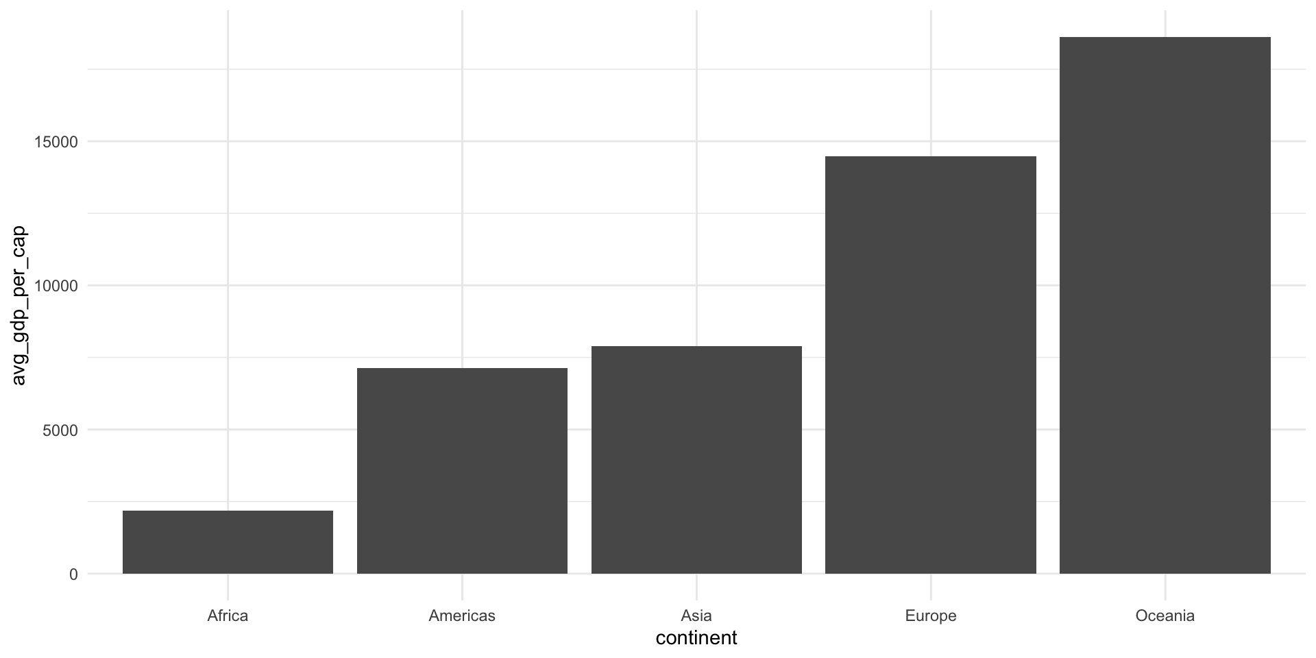

It is worth noting that there are two versions of the pipe running around. The first |> is the base pipe. This comes straight out of the box with R. You do not need to load in any packages to use it. The second, %>%, is the tidyverse pipe. To use it, you need to load in either dplyr or the magrittr package.

I have switched to using the base pipe, so that’s the one you will see in all of my code. You can use whichever you prefer!

Exercises

Use the pipe to calculate the average GDP per capita for countries in the Americas in all years including or after 2000.

Check your answer

gapminder_americas_2000 <- gapminder |> 
  filter(continent == "Americas", year > 2000) |> 
  group_by(country) |> 
  summarise(avg_gdp_per_cap = mean(gdpPercap))

gapminder_americas_2000

# A tibble: 25 × 2
   country            avg_gdp_per_cap
   <fct>                        <dbl>
 1 Argentina                   10789.
 2 Bolivia                      3618.
 3 Brazil                       8599.
 4 Canada                      34824.
 5 Chile                       11975.
 6 Colombia                     6381.
 7 Costa Rica                   8684.
 8 Cuba                         7644.
 9 Dominican Republic           5295.
10 Ecuador                      6323.
# ℹ 15 more rows

Plot your results.

Check your answer

ggplot(gapminder_americas_2000, aes(x = avg_gdp_per_cap, y = reorder(country, avg_gdp_per_cap))) + 
  geom_col() +
  theme_minimal() + 
  labs(title = "Average GDP per capita for countries in the Americas in 2002 and 2007",
       x = "Average GDP per capita (US$)",
       y = NULL) + 
  scale_x_continuous(labels = scales::label_dollar())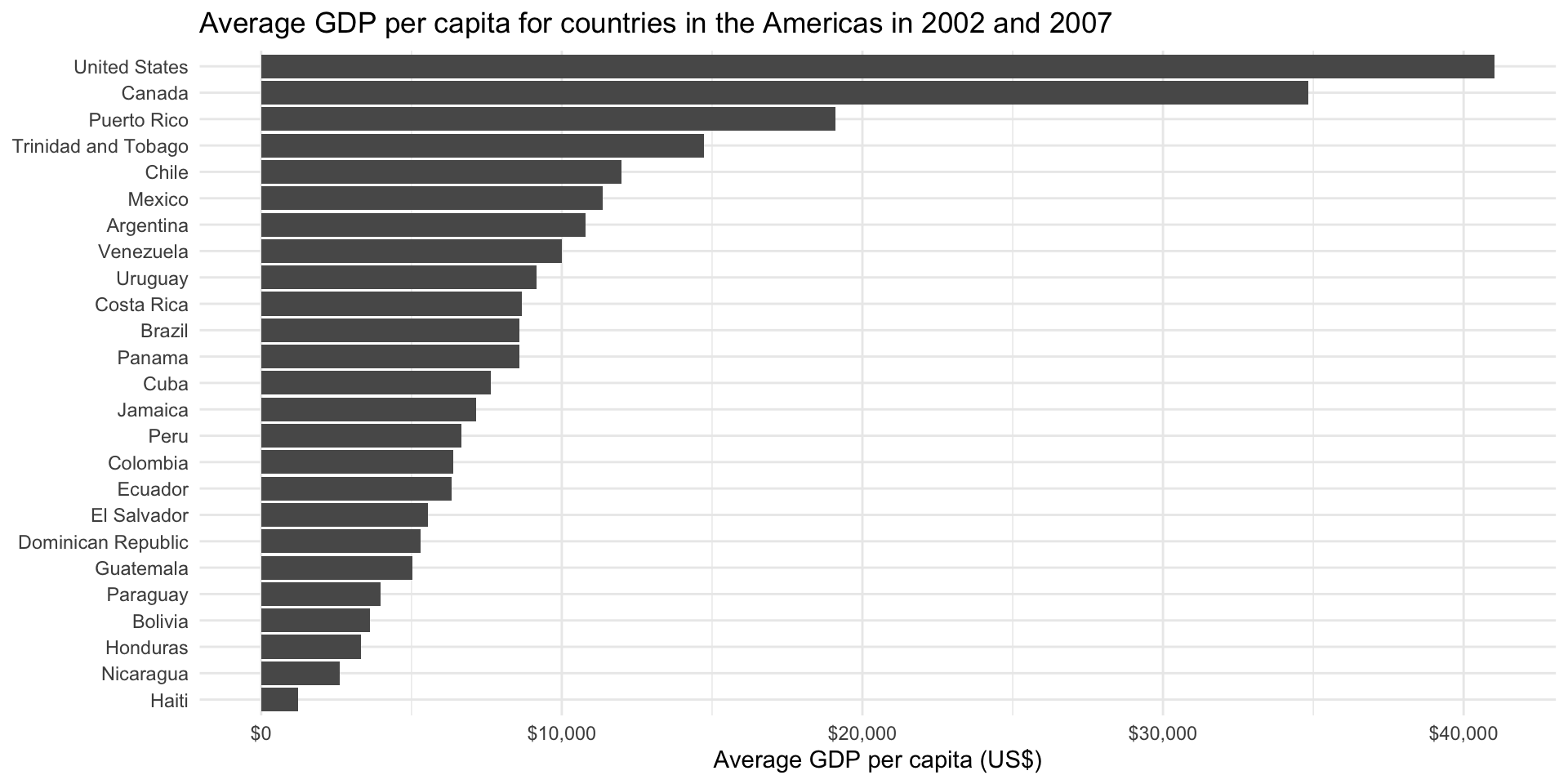

Note: Check out the scales R package for very handy formatting functions: https://scales.r-lib.org.